Field guide

LiDAR Hillshade Maps for Metal Detecting

Hillshade is where most detectorists start, but it is one of four ways of looking at the same elevation data — alongside slope, Local Relief Model, and sky-view openness. Each one hides different things and reveals different things.

In short If you are metal detecting, the point of all this is to pick your ground before you drive out to it. Raw elevation numbers rarely show anything to the eye — a foundation reduced to a few centimeters of relief is invisible at normal color scales. Hillshade, slope, Local Relief Model, and sky-view openness are all just different math applied to the same digital elevation model to exaggerate exactly that kind of small, local relief. None of them is strictly "better" — they surface different failure modes, which is why Lidarman lets you switch between them on the same search without re-running it.

Want to see these styles on your own ground? Run a search — try the free demo first, no account.

1. Hillshade

Hillshade simulates sunlight hitting the terrain from a fixed direction and renders the result in grayscale — it's the closest thing to "what the ground would look like if you stripped away every tree and building and lit it from one angle." It's the easiest style to read at a glance, because it looks like a photograph of terrain rather than an abstraction, which is why a hillshade map is usually the first thing a detectorist opens.

The catch is direction-dependence: a feature that happens to face away from the simulated sun can wash out almost completely, while an identical feature facing the light stands out sharply. A single-direction hillshade can genuinely miss things that are sitting right there. Lidarman's default composite view uses a multi-directional hillshade — the same calculation averaged over eight compass directions — specifically to reduce this blind spot, but the plain single-direction hillshade style is still useful on its own as the fastest way to get oriented in a new area before switching to something more sensitive.

2. Slope

Slope measures steepness — the rate of elevation change — at every point, independent of which way it faces. This is what makes it the right tool for not missing anything: an edge that a hillshade might hide because of unlucky lighting geometry still shows up in slope, because slope doesn't care about light direction at all.

What slope can't tell you on its own is whether an edge is the top of a rise or the bottom of a dip — a foundation wall and the ditch running next to it can produce a very similar-looking bright edge in a pure slope map. It's a detector for "something changes here," not a classifier for what kind of change it is.

3. Local Relief Model (LRM)

The Local Relief Model isolates small, local bumps and dips from the broader regional terrain trend: take the elevation model, heavily smooth a copy of it (a large-radius Gaussian blur), then subtract the smoothed version from the original. What's left is only the local deviation — a gentle hillside disappears into the subtraction, while a sharp, small-scale foundation outline or ditch survives it.

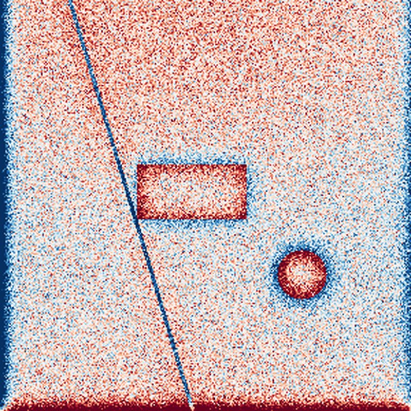
LRM is the clearest style for sorting raised from sunken at a glance, typically rendered on a diverging color scale: warm/red for higher than the immediate surroundings, cool/blue for lower. It's also the layer Lidarman's automatic candidate-detector itself analyzes (thresholded, then run through contour extraction and shape scoring) — when the tool flags a rectangular or circular candidate, LRM is what it actually looked at.

Local Relief Model of a test elevation model, raised features red and sunken features blue — A Local Relief Model on the diverging scale described above — red where the ground sits higher than its immediate surroundings, blue where it sits lower. This is the validation DEM, where the buried shapes are known in advance.

Limitation worth knowing A large, perfectly flat raised feature — a big building pad, for instance — can be nearly invisible in the interior of an LRM, because the smoothing radius only lights up the edges of a plateau much bigger than itself. The interior blends back into the smoothed baseline. If you're looking at a large flat-topped feature, cross-check it against slope or hillshade rather than trusting LRM's interior reading alone.

4. Sky-view openness

Openness measures the average horizon angle visible from each point across several compass directions — essentially, how much open sky a point on the ground can "see." Positive openness highlights convex features (mounds, walls, raised pads) that poke up above their surroundings; negative openness highlights concave features (pits, ditches, sunken paths) that dip below theirs. Because it's an average across many directions rather than one simulated light source, it doesn't share hillshade's direction-dependent blind spot.

Lidarman's default composite blends positive and negative openness with hillshade into one RGB image, which is why the composite view is a reasonable all-around default even before you know what you're looking for.

5. A practical workflow

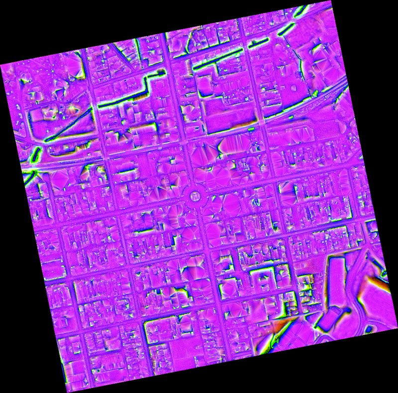
RGB composite of LIDAR terrain data over downtown Gettysburg, Pennsylvania — The composite Lidarman shows by default — positive openness, inverted negative openness and hillshade combined into one image. Real data over downtown Gettysburg, PA; building outlines, streets and the Lincoln Square circle all resolve.

Rather than picking one style and sticking with it, treat them as a sequence — this is the order that wastes the least time when you are scouting somewhere to detect:

Start with slope to catch every edge in view — this is your net, cast wide.
Switch to Local Relief to sort what you found into raised vs. sunken, and to see how the automatic detector is scoring it.
Check hillshade as a gut-check — does it look like plausible real terrain, or does it look like a rendering artifact?

This costs nothing extra: Lidarman computes all four derivative layers for every search, so switching styles is instant and doesn't re-run anything. Reading the same ground four ways before you go is what turns a hillshade map into a shortlist of places worth swinging a coil over.

6. Cheat sheet by feature type

The four shapes worth walking on, and the style that shows each one most clearly:

rectangular circular irregular

Sunken paths & old roads — Local Relief, look for a blue trail. Slope is a good backup: it shows as two parallel bright edges where the path dips in and climbs back out.
Basements & cellars — Local Relief (a blue rectangle), cross-checked against slope — steep cellar walls often read as a bright "picture frame" outline around a flatter, darker floor.
Foundations (old wall stubs) — Local Relief or the composite view, looking for a thin warm-colored outline.
Walls, berms & mounds — Composite or Local Relief — these are raised features, so they read warm on both.

More guides

Finding Ghost Towns With LIDAR — What a vanished town leaves in the ground, where the list of 16,525 of them comes from, and why the dot is only a starting point.
Detecting Near Civil War Battlefields — The protected core is off limits — the study area around it often isn't. How to tell the two apart before you knock.
Finding Old Mining Camps — 44,677 abandoned metal mines, what the camp left behind as opposed to the workings, and why the two are a short walk apart.
Finding Old Homestead Sites With LIDAR — What a vanished foundation, root cellar or filled-in farm road looks like in elevation data, and how to tell them from natural ground.
Historical Maps for Metal Detecting — Where to get old maps free, what the symbols mean, and how to line a century-old sheet up with the ground you are standing on.
Detecting Along the Westward Trails — What survives of the Oregon, California, Pony Express and Santa Fe routes, and how ruts and swales read in terrain data.
Permission and Legal Basics Before You Dig — Private land, public land and protected sites are three very different situations. General ground rules, not legal advice.

Every style above is one click away on a real search — no manual GIS work, no separate download.

Try the free demo

← Back to guides · Next: Finding Old Homestead Sites With LIDAR →